Large Language Models Are Zero-Shot Time Series Forecasters
Abstract
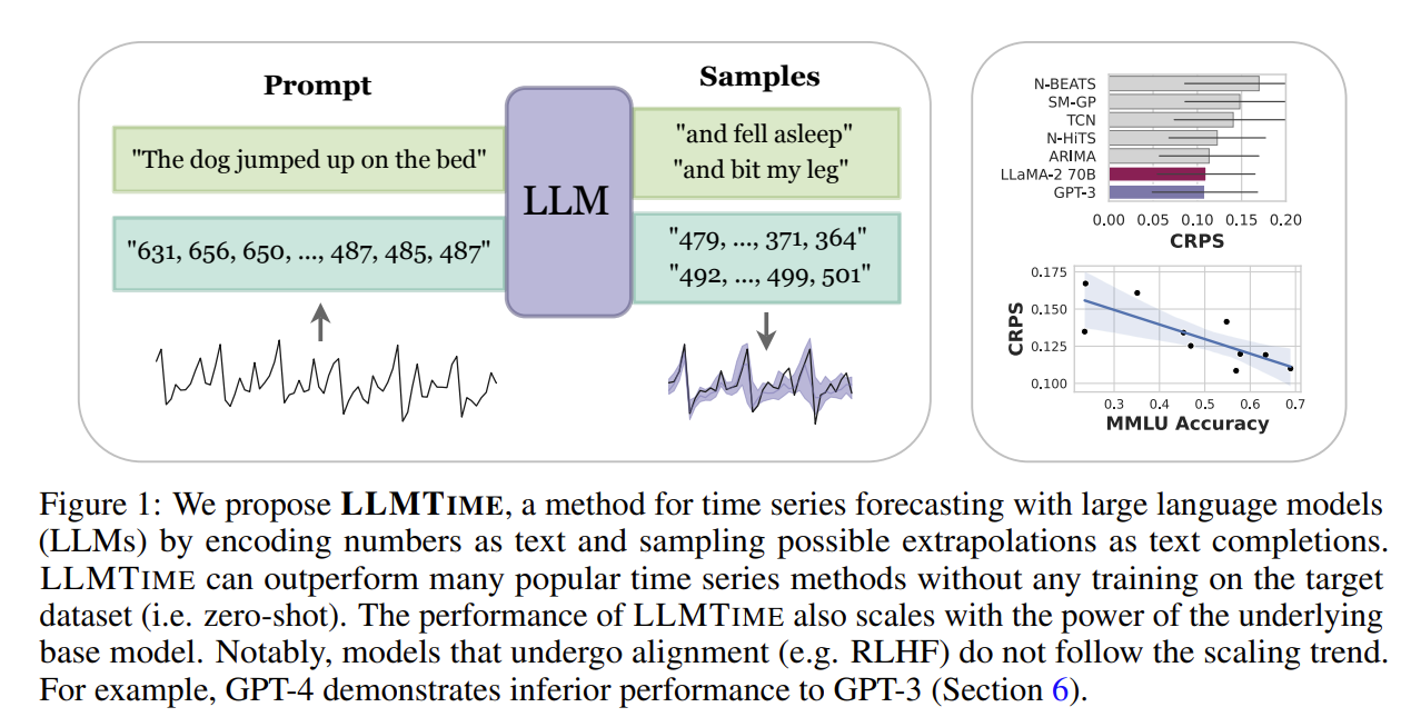
- By encoding time series as a string of numerical digits, we can frame time series forecasting as next-token prediction in text.
- This work shows that the zero-shot generalization abilities of LLMs and their preference for compressible patterns extend well beyond language understanding and can be used for time series forecasting.
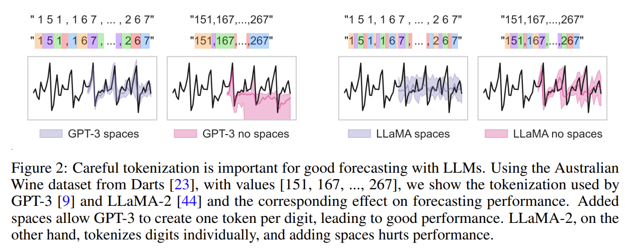
- How to effectively tokenize time series data?
- proper tokenization is extremely important
- the most common tokenization method is byte-pair encoding (BPE), which treats inputs as bit strings and assign tokens based on the rate of ocurrence in the training corpus, optimizing for shorter sequeces of tokens on average.
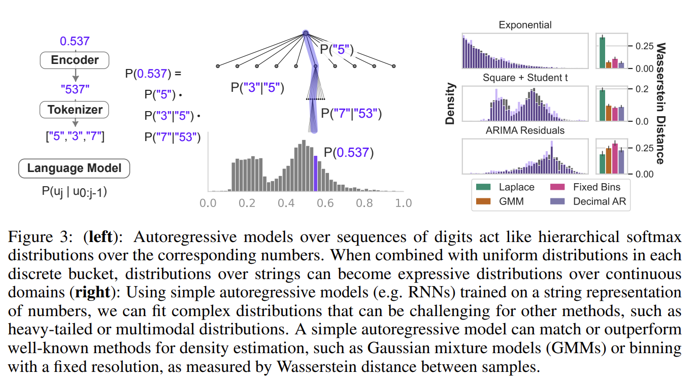
- Convert discrete distributions over tokens into highly flexible densities over continuous values
- The success of LLMs for time series could come from their abilitiy to naturally represent multimodal distributions, in conjuction with biases for simplicity and repetition, which capture salient features in many time series, such as seasonal trends.
- LLMs can also naturally handle missing data without imputation through non-numerical text
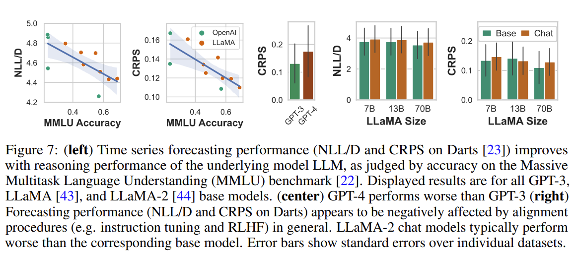
- Alignment intervention (such as RLHF) might worsen performance
Introduction
- Unlike video and audio, which typically have consistent input scales and sampling rates, aggregated time series datasets often compirse sequences from radically different sources, sometimes with missing values
- Uncertainty estimation in Financial data is specially important to extrapolate from observation containing a tiny fraction of possible information.
- There is still no consensus on an unsupervised objective for large scale pretraining for time series modeling, neither large, cohesive datasets.
- Consequently, simple time series methods (e.g. ARIMA, and linear models) often outperform deep learning methods on popular benchmarks.
- LLMTime proposes at its core to represent the time series as a string of numerical digits, and views time series forecasting as next-token prediction in text, unlocking the use of powerful pretrained models and probabilistic capacities, such as likelihood evaluation and sampling.
Background
- Proper tokenization is extremely important, and small details can have surprisingly significant effects
- LLMs are few-shot learners with incresed parameter count and training data, with zero-shot generalization though in-context learning, identifying patterns in prompts and extrapolating though the next-token prediction.
- In-context learning might emerge from extensive compression of the input data
- Compression favors learning algorithms that operate over input data with programmatic abstractions, for example context-free grammars and induction heads, which can implement copy-and-paste type operations for generating samples with highly structured syntax.
- BPE compresses numbers based on frequency of occurrence in the training data, so numbers can be broken down into awkward chunks that make learning basic numerical operations challenging
- Touvron et al. designed the LLaMA tokenizer to map numbers to individual digits, which lead to significant improvements in mathematical abilities, with small LLaMA models outperforming GPT-4
- The other challenge of applying language models to time series data is proper evaluation.
- CRPS (Continuous Ranked Probability Score)
LLMs can assign likelihoods to full sequences of time series data, and we show how a small modification to an LLM’s discrete likelihood can yield a continuous density that is useful for model comparison
- FPT finetunes a BERT encoder to perform time series forecasting
- Meta-Transformer: framework for finetuning a LM for non-text modalities, including time series.
- PromptCat proposes forecasting as a question answering with prompting
LLMTime
- Common tokenization methods like BPE tend to break a single number into tokens that don’t align with the digits, which can make arithmetic considerably more difficult
- Because decimal points are redundant given a fixed precision, we drop them in the encoding to save on context length
Rescaling $\alpha$-percentile to allow (1-$\alpha$) values to be seen by the LLM and give it the possibility of generating values higher than it has seen. Offset $\beta$. Hyperparameters tunned on validation log likelihood.
Sampling/Forecasting To forecast, draw many samples (e.g. 20) from the LLM and use the statistics of the samples at each time step to construct a point estimate (e.g. as the median) or probabilistic forecast (e.g. as quantiles). To control sampling, we use temperature scaling, logit bias, and nucleus sampling
- Continuous likelihoods Modeling sequences of individual digits has additional benefits beyond good samples.
- With $n$ digits of precision in base $B$, each sequence of $n$ digits after the decimal place corresponds to one of $B^n$ possible bins, each with width $B^{-n}$.
- Though a language model’s probability distribution is discrete, we can easily adapt it to provide a continuous density by placing a uniform distribution in each bin.
- if a given data point lies in bin k, its continuous log likelihood is $\log p(x) = log p_k + n \log B$
- finally, to obtain the likelihood $\log p(z)$ in the original input space, add a change of variables factor $\log \frac{dx}{dz}$, where $z \rightarrow x = s(z)$ is the rescaling operation in the pre-processing.
- As a result the exponentially large number of bins and exponentially small bin widths make it surprisingly efficient to represent flexible and high-resolution continuos distributions with LLMs, despite using a discrete tokenization of numbers.
- LLMs are flexible distributions Uncertainty quantification is essential to forecasting, and typical approaches to representing uncertainty in time series can be limited by misspecification. For example, fitting Gaussian or Laplace observation models perform poorly when the underlying data distribution is multimodal. GMMs (Gaussian mixture models) solve the issue but introduce additional challenges to optimization and model selection.
- We show that a LM is an underrated solution by training a small autoregressive model (AR) on a variety of one-dimensional distributions: exponential, mixture of uniform and student-t, and heavy-tailed distribution of time series prediction residuals from an ARIMA model. We evaluate these fits quantitatively by computing Wasserstein distances and compare to a Laplace observation model, a GMM trained with EM, and a logistic regression over a flat binning of the data (with a tuned bin size), each model trained on only 200 samples from the distribution. The “Decimal AR” performs extremely well, handling assymetic, multimodal and heavy-tailed distributions.
Experiments
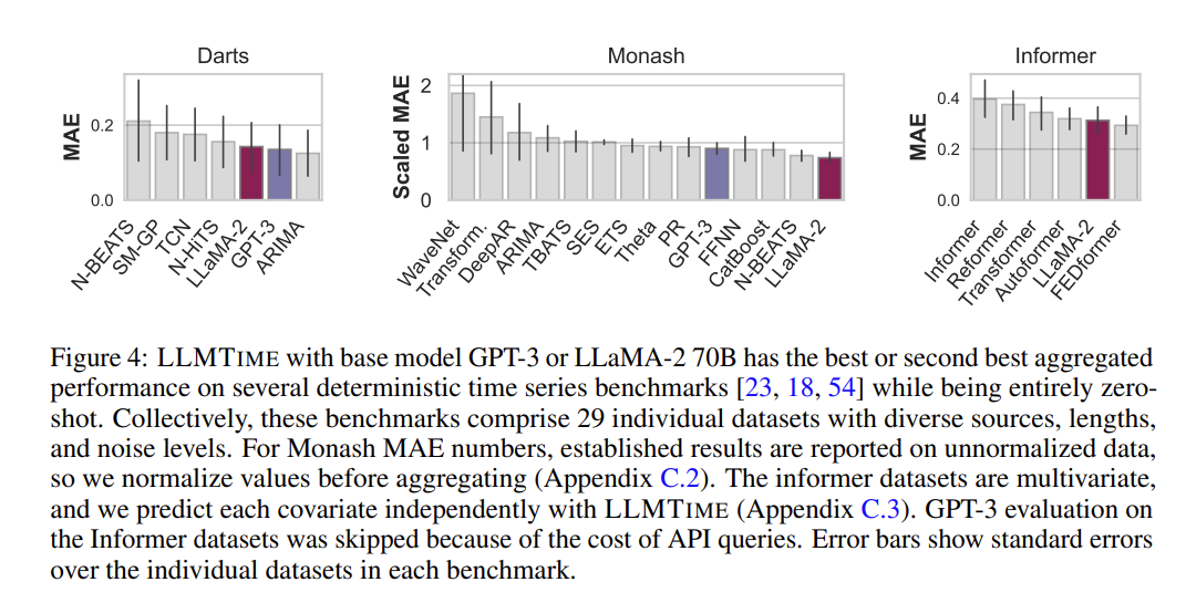
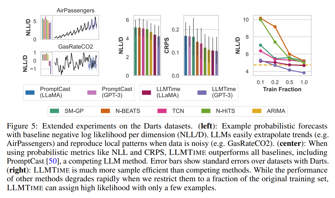
LLMTIME with base model GPT-3 or LLaMA-2 70B has the best or second best aggregated performance on several deterministic time series benchmarks while being entirely zero-shot.
For some of the longer time series, not all of the history can be fit into the context window, and hence hyperparameters implicitly capture the trade-off between higher precision and capturing a larger temporal history
- Datasets We use three benchmark datasets that are common within deep learning research and many baseline methods that accompany the benchmark datasets.
- Darts: a collection of 8 real univariate time series datasetes. Several methods are implemented in the package: TCN, N-BEATS, N-HiTS, and simple moving average models (ARIMA).
- Monash: 30 publicly available datasets along with baseline numbers for 12 forecasting models, including simple exponential smooth
- Informer: Multivariate datasets widely used for benchmarking efficient transformer models. LLMTime forecast each covariate independently.
Deterministic Results
- Probabilistic Results
Origins of Zero-shot Performance
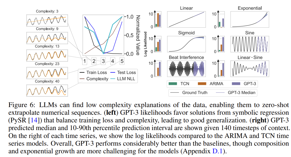
To understand why LLMs can extrapolate time series in a zero-shot manner, let’s take a step back and consider simple numerical sequences, for example $[1, 4, 9, 16, . . . ]$ or $[0, 0, 1, 0, 1, 2, 0, 1, 2, 3, . . . ]$.
For any input sequence, there are arbitrarily many generation rules that are consistent with the input (e.g. $f(x) = x^2$ for $x \in [1, 2, 3, 4, …]$), but some generation rules are overly complex and will generalize poorly
LLMs can forecast effectively because they prefer completions derived from simple rules, adopting a form of Occam’s razor prior.
To explicitly demonstrate this phenomenon, we create a synthetic example using the function $f(x) = x + cos(x)$ with additive Gaussian noise. We fit symbolic expressions to the first 70% of timesteps using PySR with symbols [”+”, “·”, “-“, “/”, “sin”, “cos”, “exp”,”square”] to identify generating rules with known complexity, quantified by the number of symbols in the regressed expression. The figure bellow shows that GPT-3 assigns the highest likelihood to symbolic regression generating rules that balance consistency with complexity.
Special Properties of LLMs.
LLMs can leverage their abilities in order to seamlessly incorporate missing data or answer questions about time series
Figure 7 (right) shows that chat versions tend to have markedly worse forecasting error than their non-chat counterparts, though still maintain trends in size and reasoning ability.
While the likelihoods of traditional methods rapidly deteriorate with corruptions, we find that LLaMA-2 70B is more resilient, and when comparing CRPS values, LLaMA-2 70B is competitive with methods that use interpolation.
Because LLMs are designed for natural language and code, we can augment the numerical time series with useful text. We can do so either by providing textual side information as inputs, or by producing textual outputs from a given time series.
An interesting question is whether GPT-4 can explain in text its understanding of a given time series, we probe this quality by providing GPT-4 the code to generate our synthetic time series, provide the values of one these time series, and then ask it to infer which of the functions produced the data in a zero-shot manner. The prediction accuracies are shown in Figure 8
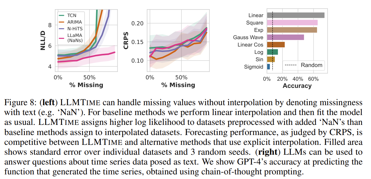
With CoT [47] prompting the model performs much better than random chance; however, its ability to identify patterns better when directly extrapolating the numerical data, suggesting that its numerical understanding is not fully connected to its textual understanding.
